
I’ve had fun over the last few days chatting with colleagues, friends, and family about the March-related weather in Charleston. See my previous blog posts to find out the background of this information. Here I’ll outline two new developments that came up today. Again, all of this pertains only to the month of March and only in Charleston SC.
(1) When do we ever use calculus, anyway?
In an e-mail yesterday, Dan Jarratt remarked that he was surprised by the result that the today-to-tomorrow temperature change had an average (mean) of +0.037 degrees Fahrenheit. In other words, given today’s high temperature, on average we expect it’ll be about 0.04 degrees warmer tomorrow. This isn’t a very big difference, as Dan remarked; it was lower than he thought it would be. This made me wonder if I too thought this was a small temperature change.
I would guess that the hottest month in Charleston is August. (That is, August is the month that has the highest average temperature.) Also, I would guess that the coldest month is six months from August, so that would mean February. Assuming that the temperature shifts in a sinusoidal fashion, we’d get a nice sine function with a period of 12 months; a local maximum in August; and a local minimum in February. This led to the following question, which I asked my Calculus students today:
When is the temperature in Charleston increasing most rapidly?
First, we had some discussion on how we could rephrase this question into one about calculus. If the temperature is increasing most rapidly, that would mean that the slope of the tangent line is its largest; this would occur halfway between February and August. We agreed that this would be the month of May. Let T(x) be the temperature at time x. Graphically, if the temperature is increasing the most rapidly, then this is where T'(x) has a local maximum, so T”(x) changes sign from positive to negative. In calculus, we call this a point of inflection: a place on the graph where the tangent line increases most rapidly (should such a place exist). Alternatively, it is where the graph changes concavity — in this case, from being concave up to concave down.
(2) What would a numerical simulation tell us?
Both my College of Charleston colleague Jason Howell and Dartmouth professor François G. Dorais suggested my predictive model wasn’t great, and
@katemath Maybe a random walk model would be better?
— François G. Dorais (@fgdorais) March 28, 2013
Thankfully, Jason was willing to help write some code toward this goal. (His code is given below, written for MATLAB, in case you’re interested!) He gathered historical averages for high temperatures for each date in Charleston, restricted to the month of March, from weather.com. The averages were computed using data from 1893 through 2013. Given that the average temperature change was +0.037F and the standard deviation of this temperature change was 8.39, we can run a number of trials to answer the question
How many days in March can we expect to be at or below their historical average temperature?
Jason’s code simulated one million different March months, given a starting temperature on March 1st of 68 degrees F. Here’s a histogram of results:
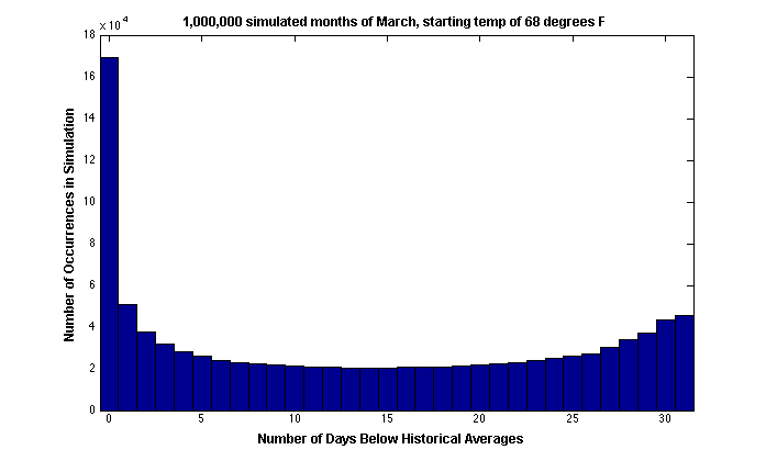 Of course, March 2013 hasn’t finished quite yet. But this histogram does tell us that if we end up with 23 or 24 days with an “at or below average” temperature, this isn’t exceedingly rare — or it isn’t as uncommon as I had thought it would be.
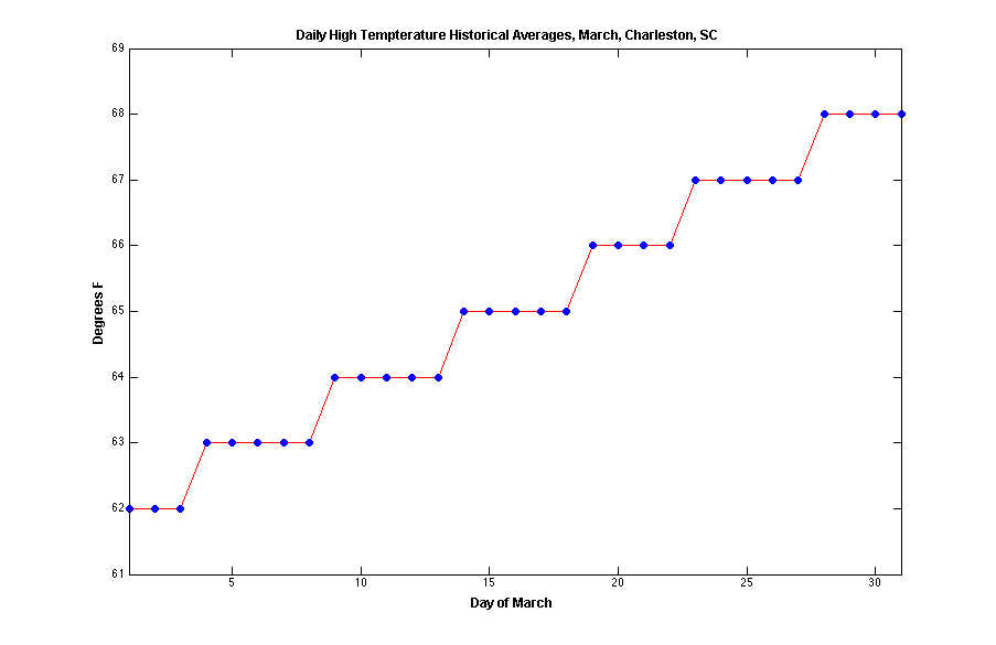
Here’s a graph of the daily average temperatures (based on the same historical data):
Jason’s Code:
function y=weatherexp(start_temp, num_trials)
%set historical averages, from weather.com
hist_avgs = [62 62 62 63 63 63 63 63 64 64 64 64 64 …
65 65 65 65 65 66 66 66 66 67 67 67 67 67 68 …
68 68 68];
%initialization
num_days=length(hist_avgs);
temp_diff = zeros(size(hist_avgs));
num_days_below = zeros(1,num_trials);
%parameters for normally distributed daily temperature changes
%from months of March from 1893 to 2012
stdev = 8.39;
avg = 0.037;
%loop over trials
for j=1:num_trials
%set temperature for start of a simulated month/week/etc.
curr_temp = start_temp;
for i=1:num_days
%get temperature change
temp_change = avg+stdev*randn(1,1);
%new temp
curr_temp = curr_temp + temp_change;
%how far from average?
temp_diff(i) = curr_temp – hist_avgs(i);
end
%count number of days below average
num_days_below(j)=sum(temp_diff<0);
%temp_diff
end
%histogram of the num_days_below data
figure
hist(num_days_below,[0:31])
y = num_days_below;
I was really puzzled by the graph above, so I spent some time trying to figure out what was happening there. Here is what I found…
In the random walk model, the change in temperature from one day to the next are independent of each other. For simplicity, I’ll assume that the average high temperature is the same every day. This can be accomplished by moving to Hawaii or San Diego, but it might be cheaper to simply adjust the way you measure temperature every day so that the average high is always your favorite number. The change in high temperature from one day to the next then has mean 0 and we assume that this change is normally distributed. Another fun fact about this model is that knowing the full history of temperatures up to today gives no more information about tomorrow’s temperature than just knowing today’s temperature.
Understanding the interaction between consecutive days is the key. What is the probability that tomorrow is cold given that today is cold? This is a conditional probability which equals the probability that today and tomorrow are both cold divided by the probability that today is cold. The probability that today is cold is 1/2. The probability that today and tomorrow are both cold is tougher. If the two temperatures were independent the probability would be 1/4, but they are not independent since tomorrow is more likely to be cold given that today is cold. However, our model tells us that the probability that tomorrow is colder than today is 1/2, independently of today’s temperature. So the probability we want is 1/4 (the probability that today is cold and tomorrow is colder) plus the probability Q that tomorrow is warmer than today but still colder than average. The value of Q varies as I will explain later. In any case, the probability that today and tomorrow are both cold is Q+1/4. So, the probability that tomorrow is cold given that today is cold is 2(2+1/4) = 2Q+1/2 and the probability that tomorrow is warm given that today is cold is -2Q+1/2. By symmetry, the probability that tomorrow is warm given that today is warm is 2Q+1/2 and the probability that tomorrow is cold given that today is warm is -2Q+1/2.
Now, let’s say that we’re given a warm/cold pattern from March 1st to March 27th. The probability that the weather actually fits this pattern is (1/2)(-2Q+1/2)^S(2Q+1/2)^(26-S) where S is the number of warm/cold switches in the pattern. To see this, work through the days in order. First, the probability that the March 1st fits the pattern is 1/2. Then, by Bayes’ formula, the probability that March 2nd fits the pattern is 1/2 times the probability that March 2nd fits the pattern given that March 1st already fits the pattern: (1/2)(2Q+1/2) if the two are the same and (1/2)(-2Q+1/2) if there is a switch from March 1st to March 2nd. The probability that March 1st, 2nd, and 3rd fit the pattern is the probability just computed times the probability that March 3rd fits the pattern given that March 1st and 2nd both fit the pattern. However, the temperature on March 1st gives no more information on the March 3rd temperature than the temperature on March 2nd already does, so the only thing that matters is whether the pattern predicts a switch between March 2nd and March 3rd. Continuing this way, until March 27th, we get the above formula.
Back to the original question, what is the probability that at least 21 of these 27 days were cold? There are lots of different patterns that match this count and they don’t all have the same probability even if they have the same count of warm and cold days. If the 6 warm days are very spread out then we can have up to twelve switches in the pattern, but if the 6 days are March 1st to March 6th, then we only have one switch from March 6th to March 7th. An exact formula seems very complicated. In any case, that does intuitively explain why having a relatively colder 27 days is more likely than haven an even balance between warm and cold since a balanced pattern is likely to have more switches.
In any case, we still need to figure out that mysterious Q. It would be fun to figure out Q by experiment, but it’s also fun to think about it theoretically. Recall that Q is the probability that today and tomorrow are both cold but tomorrow is warmer than today. If we suppose that today’s temperature T is normal with mean M and standard deviation D and that the temperature difference U from today to tomorrow is normal with mean 0 standard deviation E. We want the probability that T < M and 0 < U < M – T. Knowing the distribution, we can turn this into a pretty scary double integral. I didn't actually try to do this integral, but my computer told me that Q = (1/2pi)arctan(E/S). This is fantastic since the odds of getting a clean answer here were pretty slim at the outset. It's also neat that the standard deviations are the only thing that matter. Also, we get an indirect way to test this model by checking whether the experimental values of Q, E, S match the predictions.
I haven't figured out a good way to get the probability you want, or even a decent approximation. Maybe you (or your colleagues) have some thoughts on how to finish this?
PS: It doesn't look like you have a MathJax plugin installed. You should bug your blog admins to install it.
Thanks for the long comment, François! Will try to write longer reply later. In meantime, I think I looked into MathJax a while back; but Powers That Be said no-go because it was a security issue (re: Java?). Can’t remember details now.
You should keep bugging them: MathJax is the way to go! They’re just being silly with the security issue. It’s ridiculous for a college to deny this to their users!